
Image credit: Charlotte Edey
This comes from the file content/analysis.Rmd.
We describe here our detailed data analysis.
——-
Introduction
Our data analysis focuses on assessing the demographics of tech workers, the prevalence of mental health disorders within this group, and their attitudes and perceptions of mental health in the context of their workspace.
For demographics, we identify several variables of interest:
- Country of work
- Age
- Gender
For mental health, we identify the following variables of interest:
- Prevalence of mental health disorder, past or present
- Stigma associated with mental health
- Family history of mental health
- Perceptions of employee attitudes to mental health
- Perceptions of employee attitudes to physical health
We assess these first univariately, then in relation to each other (for variables we think may interesting to map together, such as age with gender, and perceptions of employee attitudes to mental health with those of physical health). Lastly, we look at the response patterns ond relationships of response patterns over time, made possible by combining survey data from two years, collected in 2016 and 2018.
Demographics
In the section, we will be exploring our three variables of interest: age, gender, and country of work and their relations to the big picture.
Countries
To get a sense of the geographic diversity of our response pool, we started our analysis by grouping the data from each year by country, and then generating counts per country per year using summarize(). Visualization via tables was facilitated using knitr::kable().
| Rank | Country of work (2016) | Count | Country of work (2018) | Count | |
|---|---|---|---|---|---|
| 1 | USA | 851 | USA | 312 | |
| 2 | UK | 185 | UK | 19 | |
| 3 | Canada | 74 | Canada | 8 | |
| 4 | Germany | 58 | Germany | 7 | |
| 5 | Netherlands | 47 | Poland | 6 | |
| 6 | Australia | 34 | India | 5 | |
| 7 | Sweden | 20 | Netherlands | 5 | |
| 8 | Ireland | 15 | Australia | 4 | |
| 9 | France | 14 | France | 4 | |
| 10 | Brazil | 10 | Italy | 4 |
Millions of people worldwide have mental health conditions and an estimated 1 in 4 people globally will experience a mental health condition in their lifetime. Another report from NIH says that approximately 1 in 5 U.S. adults experience some type of mental illness every year. Known for a competitive and fast-moving style of living, Americans have developed a definite stigma surrounding mental health, as well as an aversion to taking the time for proper self-care or even treatment. Not only in America, but among the developing countries, the numbers are really similar. And all the developing countries happens to be in the table above about the numbers of employees in each countries working in tech industry.
# library(tidyverse)
#
# whereFrom2016 <- combined_demographic_data %>% filter(year=="2016") %>% group_by(country_of_work) %>% count() %>% arrange(desc(n)) %>% head(n, n = 10)
# knitr::kable(whereFrom2016)
#
# whereFrom2018 <- combined_demographic_data %>% filter(year=="2018") %>% group_by(country_of_residence) %>% count() %>% arrange(desc(n)) %>% head(n, n = 10)
# knitr::kable(whereFrom2018)
Age and gender
For our age and gender analysis, we started with a per-year visualization of the participant gender breakdowns. To produce this visualization, we filtered our combined demographic data to remove any observations that contained no response for gender (value = NA). We then grouped the data by gender and year in order to calculate the counts per group using summarize. To produce the visualization, the summary tibble was simply passed to ggplot using geom_bar, with gender on the x-axis, counts on the y-axis, and bars colored by year. Position was set to “dodge” to allow for side-by-side bars plotting.
To further explore our demographic, we sought to explore the age distributions within each of these gender groups. Using a ggplot’s histogram functionality and a facet grid, we produced this visualization using a tibble filtered for non-NA gender and age observations, and grouped by gender and year.
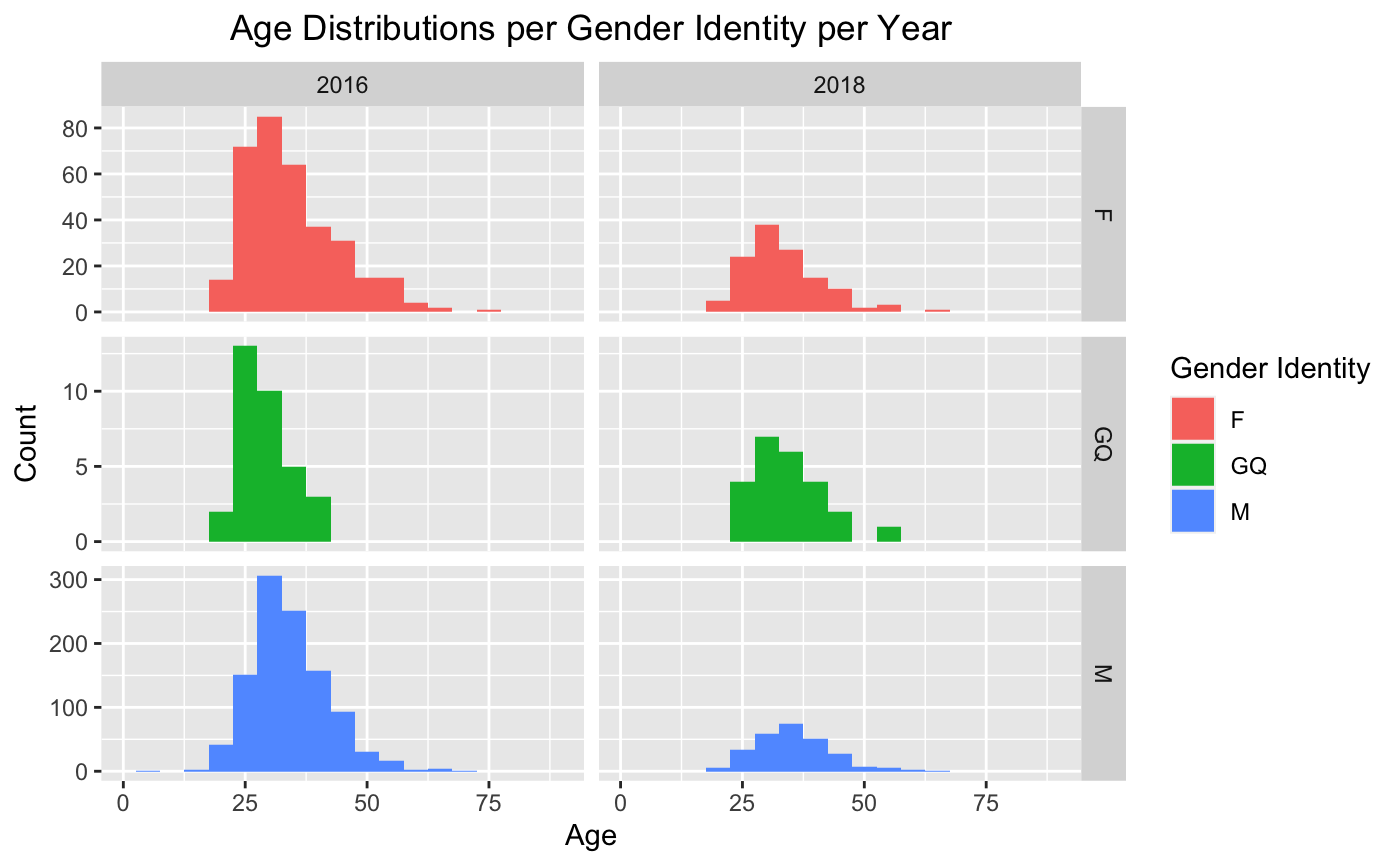
Female (49.7%) tends to seek for mental health treatments comparing to male (36.8%), according to a NIH report. Tech companies usually have a significantly bigger percentage of male workers, yet approximately 40% of responds from both year reported to suffer from a mental health problem. This is higher than the number from the United Nations on mental health issues worldwide.
Adults in the workforce are the target group of mental health disorders. SAMHSA reports 25% from the age of 26 to 49 has experienced some form of mental issues in United States. That correspond with the age range in both surveys. What we are having here is the target group for promoting mental health awareness, and there is a rising need for supporting resources in their workplace. This can be either effective counseling therapy, safe environment for discussion or better coverage in health care for mental diseases.
# age <- combined_demographic_data %>% filter(!is.na(gender)) %>% group_by(gender,year) %>% summarise(n = n()) %>% mutate(freq = n / sum(n)) %>% ungroup
# knitr::kable(age)
#
# ggplot(age, aes(x=gender, y=n, fill=year)) + geom_bar(stat='identity', position="dodge") + labs(x="Gender", y="Count") + scale_x_discrete(labels=c("Female","Queer/Undefined","Male"))
# #generate plot of age distributions per gender identity
#
# combined_demographic_data %>%
#   filter(!is.na(age), !is.na(gender)) %>%
#   ggplot() +
#   geom_histogram(aes(x = age, fill = gender), binwidth = 5) +
#   facet_grid(gender~ year, scales = "free") +
#   xlim(0, 90) +
#   labs(title = "Age Distributions per Gender Identity per Year", fill = "Gender Identity") +
#   theme(plot.title = element_text(hjust = 0.5)) +
#   xlab("Age") +
#   ylab("Count")
Exploration of mental health prevalence
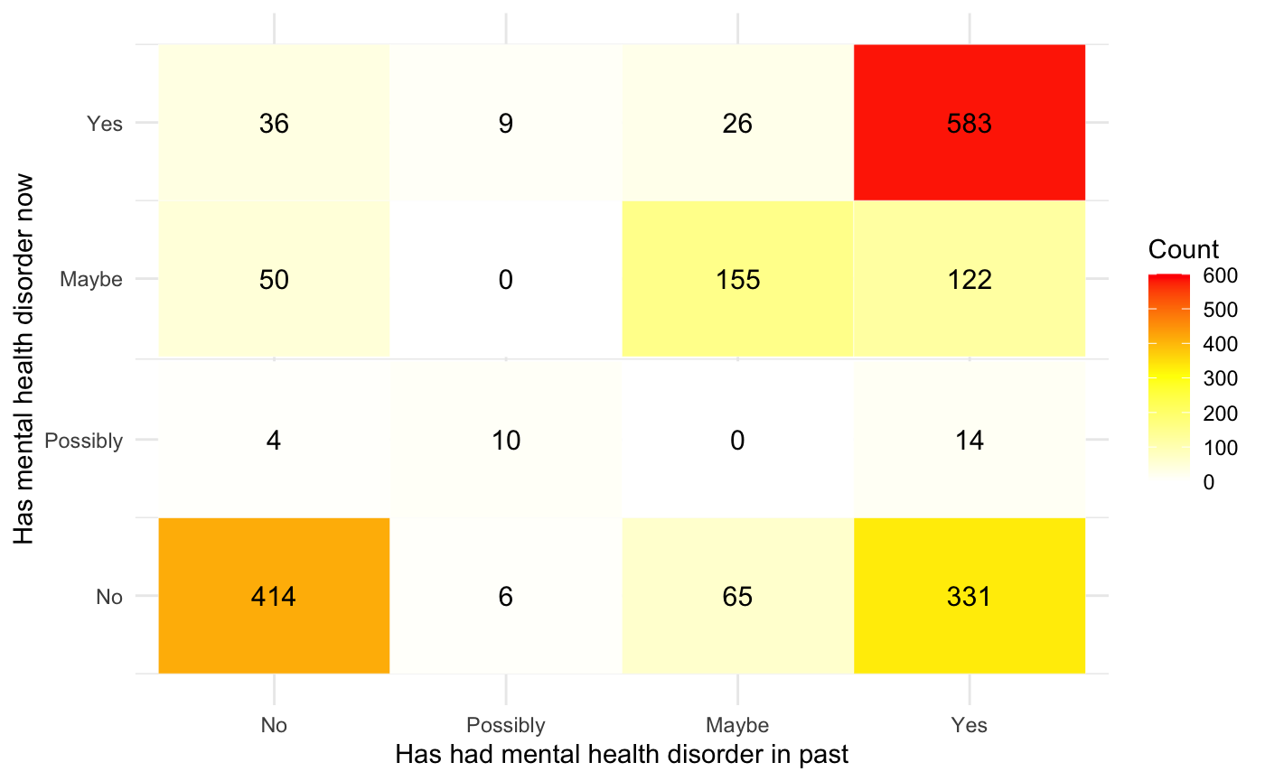
We created a heat map based on the mental health diagnosis for both 2016 and 2018 survey. There are two important things to note about this report. Approximately 17.9% people reported to recover from their disorders, and only 4.86% to have suffer from a new disorder. However, the red block on the top right shows that 31.5% continue to suffer with a mental disorders.
The table below show the percentage of people with mental health disorder by the time of the survey, divided by year.
| year | has_mhd_now | count | percentage |
|---|---|---|---|
| 2016 | Maybe | 327 | 0.2281926 |
| 2016 | No | 531 | 0.3705513 |
| 2016 | Yes | 575 | 0.4012561 |
| 2018 | Maybe | 114 | 0.2733813 |
| 2018 | No | 112 | 0.2685851 |
| 2018 | Yes | 191 | 0.4580336 |
# #summarize metrics surrounding mental health issue prevalence
#
# data2016_demographics %>%
#   filter(!is.na(had_mhd_past)) %>%
#   group_by(year, had_mhd_past) %>%
#   summarize(Count = n()) %>%
#   mutate(Percentage = Count/sum(Count))
#
# data2016_demographics %>%
#   filter(!is.na(has_mhd_now)) %>%
#   group_by(year, has_mhd_now) %>%
#   summarize(Count = n()) %>%
#   mutate(Percentage = Count/sum(Count))
#
# data2018_demographics %>%
#   filter(!is.na(had_mhd_past)) %>%
#   group_by(year, had_mhd_past) %>%
#   summarize(Count = n()) %>%
#   mutate(Percentage = Count/sum(Count))
#
# data2018_demographics %>%
#   filter(!is.na(has_mhd_now)) %>%
#   group_by(year, has_mhd_now) %>%
#   summarize(Count = n()) %>%
#   mutate(Percentage = Count/sum(Count))
Stigma Against Mental Health
A study by the World Health Organization found that between 30 and 80 percent of people with mental health issues don’t receive help. People avoid seeking treatment due to concerns about jobs and livelihood. One might face potential of unemployment and separation from society for having issues. That is the reason why stigma, prejudice and discrimination against people with mental illness is a very serious problem.
Age vs stigma
For the age and stigma analysis, a new dataset containing only age and question on the comfortable scale when talking to supervisor was created. We apply three regression models on the comfortable scale and age for 2016, 2018 and combination of both surveys. Zero will stand in for no, and one for yes. To visualize this procedure, we included graph for regressions. Since only the result for linear regression of 2018 data shows significant result, it’s the only one showing below.
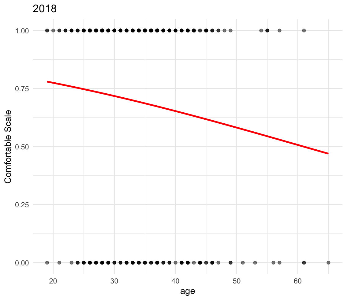
More than half of people with mental illness don’t receive help for their disorders. People are afraid of being stigmatized if they admit they need help, and the absence of a safe environment where people can discuss their issues worsen the problem. However, awareness of mental illness and the need for treatment has been growing in recent years. The younger generations have learn to be more vocal in the search for help. The 2018 analysis shows a significant correlation about the youths talking to their supervisor about their problems. There were no significant result from the 2016 or combination of both surveys, but it’s never harm to raise awareness for company to establish campaign to prevent stigma at workplace.
###Check for relationship between: "Would you be comfortable discussing mental health with your supervisor?" and age
##2018 model
#
# library(modelr)
# library(gridExtra)
#
# dat_agelm <- data2018_recode %>% filter(age >=18 & age < 80, !(is.na(age)| is.na(comfortable_discussing_mh_with_supervisors)))
#
# dat_agelm$bad_conseq <- ifelse(dat_agelm$comfortable_discussing_mh_with_supervisors == "Yes" | dat_agelm$comfortable_discussing_mh_with_supervisors == "Maybe", 1, 0)
#
# dat_agelm <- dat_agelm %>% select(age, comfortable_discussing_mh_with_supervisors , bad_conseq)
#
# age_model <- glm(bad_conseq ~ age, data = dat_agelm, family = binomial)
#
# grid <- dat_agelm %>% data_grid(age) %>% add_predictions(age_model, type = "response")
#
# p18 <- dat_agelm %>%  ggplot(aes(x = age)) +
#   geom_point(aes(y = bad_conseq), alpha = 0.5) +
#   geom_line(aes(y=pred), data = grid, color = "red", size = 1) +
#   labs(y = "Comfortable? (1/0)",
#        title = "2018") + theme(title = element_text(size = 10))+
#   theme_minimal()
#
# ##2016 model
# dat_agelm <- data2016_recode %>% filter(age >=18 & age < 80, !(is.na(age)| is.na(comfortable_discussing_mh_with_supervisors)))
#
# dat_agelm$bad_conseq <- ifelse(dat_agelm$comfortable_discussing_mh_with_supervisors == "Yes" | dat_agelm$comfortable_discussing_mh_with_supervisors == "Maybe", 1, 0)
#
# dat_agelm <- dat_agelm %>% select(age, comfortable_discussing_mh_with_supervisors , bad_conseq)
#
# age_model <- glm(bad_conseq ~ age, data = dat_agelm, family = binomial)
#
# grid <- dat_agelm %>% data_grid(age) %>% add_predictions(age_model, type = "response")
#
# p16 <- dat_agelm %>%  ggplot(aes(x = age)) +
#   geom_point(aes(y = bad_conseq), alpha = 0.5) +
#   geom_line(aes(y=pred), data = grid, color = "red", size = 1) +
#   labs(y = "Comfortable? (1/0)",
#        title = "2016" ) + theme(title = element_text(size = 10))+
#   theme_minimal()
#
# ##Both 2016 and 2018 model
# dat_agelm <- combined_data %>% filter(age >=18 & age < 80, !(is.na(age)| is.na(comfortable_discussing_mh_with_supervisors)))
#
# dat_agelm$bad_conseq <- ifelse(dat_agelm$comfortable_discussing_mh_with_supervisors == "Yes" | dat_agelm$comfortable_discussing_mh_with_supervisors == "Maybe", 1, 0)
#
# dat_agelm <- dat_agelm %>% select(age, comfortable_discussing_mh_with_supervisors , bad_conseq)
#
# age_model <- glm(bad_conseq ~ age, data = dat_agelm, family = binomial)
#
# grid <- dat_agelm %>% data_grid(age) %>% add_predictions(age_model, type = "response")
#
# pboth <- dat_agelm %>%  ggplot(aes(x = age)) +
#   geom_point(aes(y = bad_conseq), alpha = 0.5) +
#   geom_line(aes(y=pred), data = grid, color = "red", size = 1) +
#   labs(y = "Comfortable? (1/0)",
#        title = "Both 2016 and 2018") + theme(title = element_text(size = 10))+
#   theme_minimal()
#
# png("comfortable_talking_to_supervisors_vs_age.png", width = 700, height = 500)
#
# plot <- grid.arrange(
#   arrangeGrob(p16,p18, ncol=2),
#   pboth,
#   top = "\nComfort (0-1) in discussing mental health with supervisors as a function of age\n
#   Difference across years\n"
#   )
#
# print(plot)
# dev.off()
Gender vs Stigma
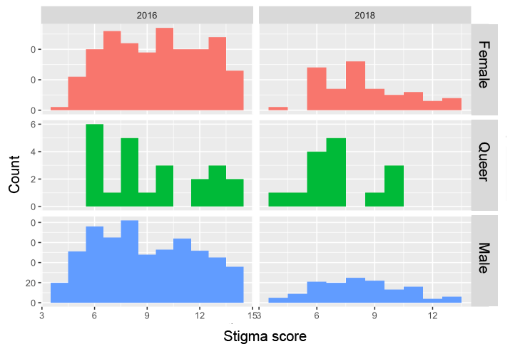
Stigma scores were created based on questions about responders’ willingness to discuss their mental health with their co-workers or supervisors. We assigned an value to each responses, ranging from lowest score for extremely comfortable discussing to highest score for the opposite. Due to the different response in every questions, response scale will differ. The range go from 1 to either 3 or 5.
We perform another analysis on stigma score and gender for both 2016 and 2018. All NAs are eliminated from the gender variables, keeping only male, female and gender queer. We use histogram plot to show the distribution of score throughout the years, by gender. We also included a table of average stigma scores.
| year | gender | Average_stigma_score |
|---|---|---|
| 2016 | F | 9.517241 |
| 2016 | GQ | 9.260870 |
| 2016 | M | 8.920608 |
| 2018 | F | 8.444444 |
| 2018 | GQ | 7.133333 |
| 2018 | M | 8.234043 |
The stigma of mental illness imposes substantial costs on both the individuals who experience mental illness and society at large, and gender has an important role. A study published on NIH shows that when a case is gender typical, responders felt more negative affect, less sympathy, and less inclination to help than a gender atypical case (Wirth & Bodenhausen, 2009). However, the table shows that stigma score did decrease for both female and gender queer, maybe in response widespread mental health awareness.
# ## how has stigma changed over time
#
# copy_combinedData <- combined_data
#
# #quantify measures of stigma
# copy_combinedData$difficulty_asking_for_mh_related_medical_leave <-
#   recode(copy_combinedData$difficulty_asking_for_mh_related_medical_leave,
#          "Very easy" = 1,
#          "Somewhat easy" = 2,
#          "Neither easy or difficult" = 3,
#          "Somewhat difficult" = 4,
#          "Very difficult" = 5)
#
# copy_combinedData$comfortable_discussing_mh_with_coworkers <-
#   recode(copy_combinedData$comfortable_discussing_mh_with_coworkers,
#          "Yes" = 1,
#          "Maybe" = 2,
#          "No" = 3)
#
# copy_combinedData$comfortable_discussing_mh_with_supervisors <-
#   recode(copy_combinedData$comfortable_discussing_mh_with_supervisors,
#          "Yes" = 1,
#          "Maybe" = 2,
#          "No" = 3)
#
# copy_combinedData$willing_to_bring_up_mh_in_interview_y_n <-
#   recode(copy_combinedData$willing_to_bring_up_mh_in_interview_y_n,
#          "Yes" = 1,
#          "Maybe" = 2,
#          "No" = 3)
#
# #generate total "stigma score" per person by summing quantified measures of
# #stigma, and plot distribution of scores per gender per year
#
# copy_combinedData <- copy_combinedData %>%
#   filter(!is.na(gender), !is.na(difficulty_asking_for_mh_related_medical_leave),
#          !is.na(comfortable_discussing_mh_with_coworkers),
#          !is.na(comfortable_discussing_mh_with_supervisors),
#          !is.na(willing_to_bring_up_mh_in_interview_y_n)) %>%
#   mutate(stigma_score = difficulty_asking_for_mh_related_medical_leave +
#                                comfortable_discussing_mh_with_coworkers +
#                                comfortable_discussing_mh_with_supervisors +
#                                willing_to_bring_up_mh_in_interview_y_n)
#
# #plot distribution of stigma scores per gender per year
#   ggplot(copy_combinedData) +
#   geom_histogram(aes(x = stigma_score, fill = gender), binwidth = 1) +
#   facet_grid(gender~ year, scales = "free")
#
# #compare averages of stigma scores per year and gender
# copy_combinedData %>%
#   group_by(year, gender) %>%
#   summarize(Average_stigma_score = mean(stigma_score))
# knitr::kable(copy_combinedData)
Linear regression prediciting mental health disorder by family history
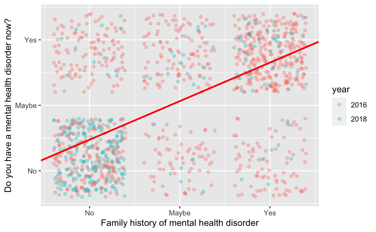
We use linear regression to model the relationship between a family history of mental health and mental health disorder: We use linear regression to model the relationship between having a family history of mental health disorder and having a mental health disorder oneself:
\[ Has\;mental\;health\;disorder = 0.238 + 0.589(family\;history\;of\;mental\;health\;disorder) \]
A scatter plot of these two variables indicates a possible linear relationship, which was further tested with the regression model. The model was significant (p-value of 2.2e-16), with an r-squared of 0.283, which indicates that 28.3% of the variation in having a mental health disorder may be explained by a family history of mental health disorder. The positive coefficients indicate a positive relationship between family and self mental health.
# convert_str <- function (sub_string) {
#   if (sub_string == 'Yes')
#     {str_num <- 1}
#   else if (sub_string == 'No')
#     {str_num <- 0}
#   else if (sub_string == 'Possibly')
#     {str_num <- 0.33}
#   else if (sub_string == 'Maybe')
#     {str_num <- 0.67}
#   else
#     {str_num <- -1}
#   return(str_num)
# }

#combined_data$num_had_mhd_past <- numeric()
#combined_data$num_has_mhd_now <- numeric()
#combined_data$num_family_history_of_mhd <- numeric()
# for (i in 1:length(combined_data$had_mhd_past))
# {
#   combined_data$num_had_mhd_past[i] <- convert_str(combined_data$had_mhd_past[i])
#   combined_data$num_has_mhd_now[i] <- convert_str(combined_data$has_mhd_now[i])
#   combined_data$num_family_history_of_mhd[i] <- convert_str(combined_data$family_history_of_mhd[i])
# }
# library(ggplot2)
# library(reshape2)
#
# # filter data for respondents who reported (1) yes family history of mhd or (0) no history
# famhist <- combined_data %>% filter(!(num_family_history_of_mhd==-1))
#
# # fit linear model
# model = lm(num_family_history_of_mhd ~num_has_mhd_now, famhist)
# mt_coef = coef(model)
#
# ggplot(famhist, aes(x= num_has_mhd_now, y= num_family_history_of_mhd)) + geom_jitter(aes(colour=year),alpha = .3) +
# geom_abline(intercept = mt_coef[1], slope = mt_coef[2], color = "red", size = 1) +
# labs(x='Family history of mental health disorder',y='Do you have a mental health disorder now?') +
# scale_x_continuous(breaks=c(0,0.5,1),labels=c( "No","Maybe","Yes"), limits=c(-0.2,1.2)) +
# scale_y_continuous(breaks=c(0,0.5,1),labels=c( "No","Maybe","Yes"), limits=c(-0.2,1.2))
#
# modelSummary <- summary(model)